Start with the Recording You Need to Keep
A storage plan is a record of assumptions about files, time and available space. Begin by listing the streams that will be saved, the recording windows and the desired history. A camera’s resolution does not supply those answers. Two systems showing equally sharp images can write different amounts of data, and a live preview can use a different stream from the recording.
For each group, record the camera or mode, video bitrate, audio treatment, daily schedule, activity basis, retention days and source of each value. Label a measured value with its sample dates. Label a manufacturer figure with the exact recording mode. Keep a hypothetical input visibly hypothetical. The resulting estimate becomes reviewable instead of looking like a measurement of equipment the calculator cannot access.
Measure Bitrate from Bytes and Time
Use original recording files from the relevant stream whenever practical. For each sample, note its exact byte count and duration. Average Mbps equals file bytes multiplied by eight, divided by seconds and then by 1,000,000. A 900,000,000-byte recording lasting 1,800 seconds averages 4 Mbps. That statement concerns this file; it does not establish a universal rate for its resolution.
Collect samples across the situations that change the scene: busy and quiet periods, daylight and darkness, movement and camera repositioning. Keep compression, frame rate and other settings unchanged during a comparison. A network meter may include live viewers and protocol traffic that are not stored in the file. An exported clip may also have been transcoded. Note those limits before treating either reading as the recorder’s storage rate.
Combine Unequal Samples with a Weighted Average
Add all sample bytes and divide by all sample seconds. Do not average their individual bitrate values unless the durations are equal. A ten-minute sample of 450 MB averages 6 Mbps. A twenty-minute sample of 450 MB averages 3 Mbps. Together they contain 900 MB over thirty minutes, so the combined rate is 4 Mbps rather than 4.5 Mbps.
Retain the separate samples even after calculating a combined number. The busy sample may be more relevant for a location whose future operating hours will be busier. Neither this simple average nor the highest observed rate provides a statistical confidence interval. Store the observed range, explain what conditions it covers and document important conditions that have not yet been sampled.
Account for Audio and Every Stored Stream
Check what a bitrate describes. A complete-file measurement normally includes the audio and container data in that file. Adding an audio estimate again would count that part twice. A video-only stream specification, in contrast, needs a separate audio amount when audio is recorded. Convert kbps to Mbps by dividing by 1,000 before adding the two rates.
Some recorders retain a continuous low-rate stream and higher-rate event clips. Calculate the time and rate of each stored stream separately, then add their bytes. Count independent audio files, thumbnails or other material only when they are actually retained and not already represented. Avoid assuming that all cameras share the same settings merely because they connect to the same NVR.
Use Recording Activity Within the Scheduled Window
Scheduled hours and active recording are separate inputs. Eight scheduled hours with 25% activity mean two recorded hours per day in this model. Continuous recording uses 100% activity even during a quiet scene. Event recording needs the observed duration actually saved, including pre-event and post-event footage. Nearby triggers can overlap and form longer recordings.
An average calculated over saved segments describes active recording time. Combine that with an observed active fraction of the schedule. A whole-day average made from total daily bytes already includes pauses; multiplying it by another activity reduction would underestimate storage. State which approach your measurement uses. With no useful observation, calculate a continuous scenario as a visible comparison rather than inventing a motion-saving percentage.
Build the Base Data Total Before Any Reserve
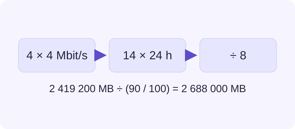
For matching cameras, multiply combined bits per second by the camera count and by recorded seconds, then divide by eight. One Mbps for twenty-four hours produces 10.8 decimal GB. Four cameras at 4 Mbps, recording continuously for fourteen days, therefore produce 2,419.2 GB before separately counted audio and overhead. Retention is the duration you choose to model, not a legal recommendation.
Adding 64 kbps of audio to each of those four video streams adds 38.7072 GB over the same period. The combined total becomes 2,457.9072 GB. Those values assume audio follows the same recording schedule. A different audio schedule needs its own calculation. Keep enough precision during arithmetic and round only the displayed result, so small early rounding errors do not grow across many cameras.
| Part | Recorded Data |
|---|---|
| Video at 4 Mbps per camera | 2,419.2 GB |
| Audio at 64 kbps per camera | 38.7072 GB |
| Combined | 2,457.9072 GB |
Separate a Margin from a Final-Volume Reserve
An added margin multiplies the data total. Adding 20% to 100 GB gives 120 GB. A reserved fraction describes the final volume instead. Keeping 20% of that volume outside the recording budget requires 100 divided by 0.8, or 125 GB. Both calculations are valid for their stated purpose, but they do not mean the same thing.
For the combined example above, a 10% final-volume reserve means 2,457.9072 divided by 0.9, or 2,731.008 GB of usable volume before that reserve. Do not add another formatting adjustment simply because a system displays GiB or TiB. Decimal GB and binary GiB express the same bytes differently. Actual file-system use, recorder databases and RAID parity are separate uses that need their own accounting.
Show Uncertainty as Scenarios, Not False Precision
Change uncertain inputs one at a time and keep the evidence beside each version. Four cameras averaging 3 Mbps instead of 4 Mbps would use 1,814.4 GB for the same continuous fourteen-day window, without audio. At 5 Mbps they would use 3,024 GB. These are conditional scenarios, not certified lower and upper bounds on future recording.
Separate uncertainty in rate from uncertainty in activity and duration. A quiet-week measurement cannot settle a busy-season question. A larger reserve may cover a chosen contingency, but it does not prove that an unobserved event will fit. Mark which result is based on measured data and which uses an assumed rate, then replace assumptions as representative recordings become available.
Adapt the Method to a Photo and Video Shoot
For a finite shoot, start from planned recorded minutes rather than the finished edit length. Add the expected photo count multiplied by the measured mean file size per shutter press. RAW+JPEG pairs should use their combined size. Eight hundred exposures at 30 MB plus twenty minutes of 100 Mbps video total 39 GB; a 20% added allowance makes 46.8 GB.
Check camera card space separately from the editing workspace. Proxies, separate sound, caches and exports may live elsewhere and need their own entries. A backup duplicates selected material on a separate destination; it is not merely spare capacity on the original card. Compare the calculated shoot budget with the card’s current free space and the camera maker’s supported recording modes.
Validate the Recorder and Keep the Evidence
Check supported disk sizes, drive bays, recording bandwidth, channel limits and the capacity left by the selected array configuration. Raw disks are not the recording volume. A usable RAID calculation helps with capacity, but it does not certify sustained performance or protect against accidental deletion, theft or a recorder-wide failure. Keep an independent, tested recovery plan for footage that must survive such events.
After commissioning, log daily growth, recording gaps and the oldest playable segment for each camera. Test playback and an export using authorized footage, then check the same dates after the intended retention period. Free space alone does not prove the history exists. Save the configuration, sample log, calculation version and verification date together. Revisit them after changing streams, schedules or hardware; do not label projected retention as observed until that history has actually been checked.